Part 4
Due Date Mar 13 11:59:59 PM
Discussion slides
Discussion slides can be accessed from here.
Before getting started
Here are some clarifications that might help you in formulating the structure of your project -
ConstantPropAnalysis.cppYour first task for this part is to implement an inter-procedural modified global variables analysis. For each function, your analysis describes which global variables may be modified. This analysis operates on LLVM IR.
In this part you will implement a modified global variables (mod) analysis. The results of the MOD analysis will be used in the flow functions of the ConstPropAnalysis
Mod Analysis
Your first task for this part is to implement an inter-procedural modified global variables analysis. For each function, our analysis pass describes which global variables may be modified. This analysis pass operates on LLVM IR.
Implementation hint - Just to make things less complicated, for now, we will store all the variables that adhere to the conditions mentioned below irrespective of them being global or not. While printing out the information in the print function for ConstantPropAnalysis, we will keep an additional condition so that we only print out the global variables.
May-point-to set (MPT)
We are going to be implementing a very conservative mod analysis. The mod analysis will make use of a very simple may-point-to analysis which can be described as follows:- There exists a global set, the MPT set, i.e. there's only one MPT set in the module, not one for each function.
- If you read the address of any variable (for example X = &Y), the variable must be added to the MPT set.
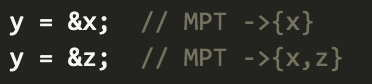
- If you encounter an operand in a function that is being passed by reference, you need to add it to the MPT set as well.
function foo (....&operand....){}This implies that the operand is passed by reference to the function and therefore can be pointed/modified by a variable inside the function. Therefore, we will add this operand to the MPT set.
One question you might have at this point is how do I get the operands passed by reference?
Ans - We will leverage theUse&data type provided by LLVM. For any given call instruction I, you can get the operands that were passed by reference as follows -
for (Use& operand : I.operands()) {}
Data Structure for MPT
You can use a global set of Value* to store the information:std::set <Value*> MPT;After you calculate the MPT set, you will use it in your mod analysis.
LMOD and CMOD sets
LMOD stands for Local MOD and CMOD stands for Callee MOD. Trivially, the variables that may be modified in the body of a function are -- the variables modified locally in the body of the function by any instruction excluding calls
- and the variables modified in the body of other functions by calls.
-
If an instruction modifies a global variable, the global variable must be added to LMOD,
glob = ....
Add glob to the LMOD set for that function -
If an instruction modifies a dereferenced pointer in any given function F, i.e.,
*var = ...., you'll need to add the subset of MPT containing GlobalVariables to the LMOD for that particular function. (This is the condition where MPT needs to be added to MOD as mentioned in before getting started section)
Note: Since this is a MAY analysis we can choose to not remove any thing from our Infos. The analysis will be correct but may be not very precise.
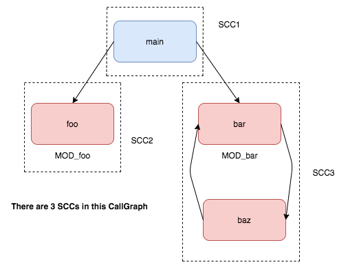
Now we come to CMOD, the tricky part. To calculate CMOD, you will need to know the caller-callee relationships between functions. This information can be obtained from the call graph. Every function's CMOD is the union of all of its callee's MODs.This is where you'd have ideally written a new worklist algorithm and kept on pushing the callers and callees on the stack till the we reached a fixed point (This was how it was discussed in the lecture).
But instead of writing a new worklist algorithm or changing the one we have in
231DFA.h, we will use the concept of strongly connected components here and that is precisely the reason why we use the CallGraphSCCPass, because it gives us those strongly connected components.
More information on SCC can be found here. You don't need to worry about the actual details of SCC but all you need to remember is that there's a smart way to start iterating over your functions and the SCC pass gives you the necessary APIs to do that.
CallGraphSCCPass
The underlying structure for this pass is the same as any other pass you've written till now. You have yourdoInitialization method, your runOnSCC method(which is analogous to the runOnFunction method of a function pass), and the doFinalization method.
Detailed information about this pass can be found on LLVMs documentation here
The following calculation are supposed to be made in each of the methods -bool doInitialization(CallGraph &CG)
You'll build your MPT and LMOD data structures in this method. Just one run across the call graph is sufficient for calculating them
Remember that since you have the call graph with you, you have access to all the functions in the module.
bool runOnSCC(CallGraphSCC &SCC)
You'll build your CMOD data structures in this method
The
SCCwill give you all the caller-callee relationship that you can use to calculate the MOD for the functions in your module. You'll get theLMOD[caller]and then you'll get theMOD[callee]. The union of these two things isMOD[caller]bool doFinalization(CallGraph &CG)
The above two functions would have built the MOD map and MPT set.
This is the function where you'll iterate over the entire call graph and call the worklist algorithm that you had written in
231DFA.hto do the Constant Prop Analysis on each function and print the analysis results.
More Info on SCC
The SCC data structure contains the CallGraphNode. The CallGraphNode further provides you access to the function that is present in that CallGraphNode. To access the function present in a CallGraphNode, use the getFunction() method on it.
Once you get the Function from the CallGraphNode, you need to find the Callee(s) of that function, if any, and union the MODS.
One special case I want to draw your attention towards is -
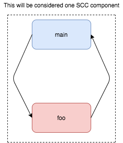
Notice that in this case the MOD[main] = MOD[foo], otherwise we would never reach a fixed point
This basically implies that the MOD of all the functions within one specific SCC has to be the same.Call Graph
A call graph is a graph which describes the caller-callee relations. LLVM builds a call graph for a given module, which consists of nodes representing functions in the module. Edges in the graph are directed edges from caller functions to callees. You can read more about LLVM's call graphs here.The following functions might be useful when working with a callgraph -
CG.getModule().getGlobalList()- gives a list of GlobalVariables in the call graphCG.getModule().functions()- gives you a list of all the functions in the call graph
Data Structure for MOD
You can use a map withFunction* as key and GlobalVariable set as the valuestd::unordered_map<Function*, std::set<GlobalVariable*>> MOD;
Directions
To implement the mod analysis, you need to
- Calculate a MPT set for your module;
- Calculate an LMOD set of each function in your module;
- Iteratively calculate CMOD until you reach a fixed set.
- You may assume no composite-typed variables exist in the module. For example, you don't need to worry about arrays, structs, unions, etc.
- You should be writing test cases as you design this analysis pass to make sure you're calculating every set correctly.
- You will only be using the information you calculate here (the final MOD set for each function) in your next analysis, so there's no need to print any output.
Constant Propagation Analysis
In part 4, you will also need to implement a constant propagation analysis based on the data-flow analysis framework you used earlier in the project. The analysis describes at each point in the program which global variables must be a constant value, and their corresponding constant values.
Lattice
For this analysis, you will map every global variable to a single constant value, top (not constant), or bottom (all constants). As discussed in lectures earlier in the class, using a lattice of height 2 for every variable guarantees termination in the worklist algorithm.
Flow Functions
Again, we'll be similar same flow functions to the flow functions described in lecture. You should use LLVM's ConstantFolder to fold in unary and binary expressions with constant operands into a constant. You need to include #include "llvm/IR/ConstantFolder.h" for ConstantFolder to work
To simplify the analysis, after a call instruction we set all variables in the callee's MOD set to top (we assume every variable in MOD was modified to some non constant value).
Also, when we encounter an instruction which modifies a dereferenced pointer, set all variables in MPT to top.
NOTE - We will not be providing explicit flow function definitions for this analysis like we did in the previous parts. It is your responsibility to come up with the flow functions yourselves. To check if your understanding is correct, run it against the reference solution provided or if you really can't figure out the flow function for any instruction, discussions on Piazza/OHs are always welcome
For the ConstantProp analysis, you only need to consider the following IR instructions:
- All the instructions under binary operations;
- All the instructions under binary bitwise operations;
- Instructions under unary operations;
- load;
- store;
- call;
- icmp;
- fcmp;
- phi;
- select.
Data Structures
These following data structures can be used while implementing your constant prop analysis :
enum ConstState { Bottom, Const, Top };- enum to store which state the operand belongs tostruct Const { ConstState state ; Constant* value; };- struct for storing info about a constant valuetypedef std::unordered_map<Value*, struct Const> ConstPropContent;- the map used by ConstPropInfo for storing the content
You are in no way limited to using these data structures, if you have a better design in mind, please feel free to use that. If you do decide to use this design then you don't need to worry about the IndexToInstr and InstrToIndex map. You can directly store the instructions as is
Directions
To implement the constant propagation analysis, you need to create
class ConstPropInfoinConstPropAnalysis.cpp: the class represents the information at each program point for your constant propagation analysis. It should be a subclass ofclass Infoin231DFA.h;class ConstPropAnalysisinConstPropAnalysis.cpp: this class performs a constant propagation analysis. It should be a subclass of DataFlowAnalysisflowfunctionneeds to be implemented in this subclass according to the specifications above;- A CallgraphSCC/Module pass called
ConstPropAnalysisPassinConstPropAnalysis.cpp: This pass should be registered by the name cse231-constprop. After processing a function, this pass should print out the constant propagation information at each program point tostderr. The output should be in the following form:
whereEdge[space][src]->Edge[space][dst]:[glob1]=[val1]|[glob2]=[val2]| ... [globK]=[valK]|\n[src]is the index of the instruction that is the start of the edge,[dst]is the index of the instruction that is the end of the edge.[globi]is a string representation of the ith global variable (the variable name).[vali]is the string representation of the ith value (⊤, ⊥, or a constant value). - You may assume that only C functions will be used to test your implementation.
- You may assume that inttoptr never appears in any test cases.
Testing
To help you test your code, we provide our solution contained in the docker image. All solutions have been compiled in a module named "231_solution.so". Our constant propagation analysis solution is registered with the same name (cse231-constprop). For example, to run the constant propagation solution, type
opt -load 231_solution.so -cse231-constprop < input.ll > /dev/null Moreover, you are also required to write 10 test cases of your own, ideally, covering all the instruction types mentioned above and make sure that the output produced by your solution is the same as that you the solution provided to you. You'll be required to submit these test cases and you'll be graded on them. Submission instructions can be found in the section below
Turnin Instructions
You will turn in your submission in Gradescope. As soon as you submit, your code will be auto-graded and you should have your grade and some feedback within a few minutes. You are allowed to submit as many times as you want until the deadline.Grading
Your submission will be graded against some benchmarks we developed which satisfy all the requirements. Unlike part 1, partially correct submissions will receive partial credit (grading strategy presented below). The order of your output does not matter - This includes the line order, as well as the order within a line. But make sure you follow the output form to the letter (no extra spaces/tabs, printed in stderr, no extra output). The autograder attempts to clean the extra output (if any), but do not rely on that.Submission Directions
- Same as with previous parts, you have to submit all source files necessary to compile your passes.
- Since you are providing a CMakeLists.txt file, your source code files can have any name you want. But the LLVM module must be named
submission_pt4and the pass need to be namedcse231-constprop
Submitting Testcases
You are required to submit a total of 10 test cases in a zipped file named tests.zip to the LLVM Project - Part 4 (TESTS) assignment. Within that zipped folder you should have a total of 10 test cases with the naming format -test_{i}.c or test_{i}.cpp In conclusion, within the zipped folder named tests.zip you should have the following test files - test_1.cpp, test_2.cpp......test_10.cpp
We will test these cases against our solution as well as your submission and grade you based on the output produced.
This is worth 10% of this assignment's grade
(90% for your MOD and ConstProp Analysis and 10% for your test cases).