> {-# LANGUAGE DeriveFunctor #-}
> {-@ LIQUID "--no-termination" @-}
> module Monads  where
>
> import Data.Map hiding (map)
>
> -- instance Functor     ST0 where
> instance Applicative ST0 where
> -- instance Functor     (ST s) where
> instance Applicative (ST s) where
Formatted version of the lecture notes by Graham Hutton, January 2011
The functional programming community divides into two camps:
“Pure” languages, such as Haskell, are based directly upon the mathematical notion of a function as a mapping from arguments to results.
“Impure” languages, such as ML, are based upon the extension of this notion with a range of possible effects, such as exceptions and assignments.
Pure languages are easier to reason about and may benefit from lazy evaluation, while impure languages may be more efficient and can lead to shorter programs.
One of the primary developments in the programming language community in recent years (starting in the early 1990s) has been an approach to integrating the pure and impure camps, based upon the notion of a “monad”. This note introduces the use of monads for programming with effects in Haskell.
Monads are an example of the idea of abstracting out a common programming pattern as a definition. Before considering monads, let us review this idea, by means of two simple functions:
inc	       :: [Int] -> [Int]
inc []     =  []
inc (n:ns) =  n+1 : inc ns

sqr	       :: [Int] -> [Int]
sqr []     =  []
sqr (n:ns) =  n^2 : sqr ns

inc = map (+ 1)
sqr = map (^ 2)

tincr = tmap (+ 1)
tsqr  = tmap (^ 2)
incr :: BST k Int -> BST k Int incr Emp = Emp incr (Node k v l r) = Node k (v + 1) (incr l) (incr r)
sqrr :: BST k Int -> BST k Int sqrr Emp = Emp sqrr (Node k v l r) = Node k (v ^ 2) (incr l) (incr r)
foog :: (a -> b) -> Maybe a -> Maybe b tmap :: (a -> b) -> BST k a -> BST k b map :: (a -> b) -> List a -> List b
>
> incr :: (Transformable blob) => blob Int -> blob Int
> incr = tx (+ 1)
> -- square = tx (^ 2)
>
> data BST k v = Emp | Nod k v (BST k v) (BST k v) deriving (Show)
>
> class Transformable c where
>   tx :: (a -> b) -> c a -> c b
>
> instance Transformable (BST k) where
>   tx _ Emp           = Emp
>   tx f (Nod k v l r) = Nod k (f v) (tx f l) (tx f r)
>
> instance Transformable Maybe where
>   tx _ Nothing  = Nothing
>   tx f (Just x) = Just (f x)
>
> instance Transformable [] where
>   tx _ []     = []
>   tx f (x:xs) = f x : tx f xs
Both functions are defined using the same programming pattern, namely mapping the empty list to itself, and a non-empty list to some function applied to the head of the list and the result of recursively processing the tail of the list in the same manner. Abstracting this pattern gives the library function called map
map         :: (a -> b) -> [a] -> [b]
map f []     = []
map f (x:xs) = f x : map f xs
using which our two examples can now be defined more compactly:
> inc = map (+1)
> sqr = map (^2)What is the type of foo defined as:
data Maybe a = Just a | Nothing> foog :: (a -> thing) -> Maybe a -> Maybe thing
> foog f (Just x) = Just (f x)
> foog f (Nothing) = NothingMaybe a(a -> b) -> Maybe a -> Maybe b(a -> b) -> a -> Maybe b(a -> b) -> Maybe a -> b(a -> Maybe b) -> Maybe a -> Maybe b
mapThe same notion of mapping applies to other types, for example, you can imagine:
map :: (a -> b) -> Maybe a -> Maybe bor
map :: (a -> b) -> Tree a -> Tree bor
map :: (a -> b) -> IO a -> IO bWhich of the following is a valid
iomap :: (a -> b) -> IO a -> IO b
iomap f x = f x             -- a

iomap f x = do f x          -- b

iomap f x = do y <- f x     -- c
               return y

iomap f x = do y <- x       -- d
               return (f y)

iomap f x = do y <- x       -- e
               f y
For this reason, there is a typeclass called Functor that corresponds to the type constructors that you can map over:
class Functor m where
  fmap :: (a -> b) -> m a -> m b
Note: The m is the type constructor, e.g. [] or IO or Maybe
We can make [] or IO or Maybe be instances of Functor by:
instance Functor [] where
  fmap f []     = []
  fmap f (x:xs) = f x : fmap f xs
and
instance Functor Maybe where
  fmap f Nothing  = Nothing
  fmap f (Just x) = Just (f x)
and
instance Functor IO where
fmap f x = do {y <- x; return (f x)}map to Many ArgumentsWe can generalize map to many arguments.
With one argument, we call it lift1
lift1           :: (a1 -> b) -> [a1] -> [b]
lift1 f []      = []
lift1 f (x:xs)  = f x : lift1 f xs

lift2           :: (a1 -> a2 -> b) -> [a1] -> [a2] -> [b]
lift2 f (x1:x1s) (x2:x2s) = f x1 x2 : lift2 f x1s x2s
lift2 f _        _        = []

lift2           :: (a1 -> a2 -> b) -> Maybe a1 -> Maybe a2 -> Maybe b
lift2 f (Just x1) (Just x2) = Just (f x1 x2)
lift2 f _        _          = Nothing
You can imagine defining a version for two arguments
lift2 :: (a1 -> a2 -> b) -> [a1] -> [a2] -> [b]
lift2 f (x:xs) (y:ys) = f x y : lift2 f xs ys
lift2 f _      _      = []
and three arguments and so on
lift3 :: (a1 -> a2 -> a3 -> b) -> [a1] -> [a2] -> [a3] -> [b]or
lift2 :: (a1 -> a2 -> b) -> Maybe a1 -> Maybe a2 -> Maybe b

lift2 f (Just x) (Just y) = Just (f x y)
lift2 _ _        _        = Nothing


lift3 :: (a1 -> a2 -> a3 -> b)
      -> Maybe a1
      -> Maybe a2
      -> Maybe a3
      -> Maybe b
or
lift2 :: (a1 -> a2 -> b) -> IO a1 -> IO a2 -> IO b
lift2 f x1 x2 = do a1 <- x1
                   a2 <- x2
                   return (f a1 a2)


lift3 :: (a1 -> a2 -> a3 -> b)
      -> IO a1
      -> IO a2
      -> IO a3
-> IO bclass Functor f => Applicative f where
pure :: a -> f a
(<*>) :: f (a -> b) -> f a -> f b
pure :: a -> BLOB a
<*> :: BLOB (a -> b) -> BLOB a -> BLOB b
lift2 :: (a1 -> a2 -> b) -> BLOB a1 -> BLOB a2 -> BLOB b
lift2 f x1s x2s = pure f <*> x1s <*> x2sFor this reason, there is a typeclass called Applicative that corresponds to the type constructors that you can lift2 or lift3 over.
liftA  :: Applicative t => (a -> b) -> t a -> t b

liftA2 :: Applicative t => (a1 -> a2 -> b) -> t a1 -> t a2 -> t b

liftA3 :: Applicative t
       => (a1 -> a2 -> a3 -> b)
       -> t a1
       -> t a2
       -> t a3
       -> t b
Note: The t is the type constructor, e.g. [] or IO or Maybe or Behavior.
Consider the following simple language of expressions that are built up from integer values using a division operator:
> data Expr1 = Val1 Int
>            | Div1 Expr1 Expr1
>            | Boo1 Expr1 Expr1 Expr1
>              deriving (Show)
Such expressions can be evaluated as follows:
e1 >>= 1 -> e2 >>= 2 -> e3 >>= 3 -> e4 >>= 4 -> stuff
do n1 <- e1 n2 <- e2 n3 <- e3 n4 <- e4 stuff
> eval2 :: Expr1 -> Maybe Int
> eval2 (Val1 n)        = Just n
> eval2 (Div1 e1 e2)    = do { n1 <- eval2 e1;
>                              n2 <- eval2 e2;
>                              safeDiv n1 n2
>                            }
>
> eval2 (Boo1 e1 e2 e3) = do n1 <- eval2 e1
>                            n2 <- eval2 e2
>                            n3 <- eval2 e3
>                            safeDiv (n1 + n2) n3
>
> eval1              ::  Expr1 -> Int
> eval1 (Val1 n)     =  n
> eval1 (Div1 x y)   =  eval1 x `div` eval1 y
> eval1 (Boo1 x y z) =  (eval1 x + eval1 y) `div` eval1 z
>
> {-
> eval2 (Div1 (Val1 6) (Val1 2))
>    == eval2 (Val1 6) >>= ...
>    == Just 6 >>= (\n1 -> ...)
>    == (\n1 -> ...) 6
>    == (eval2 e2 >>= \n2 -> safeDiv 6 n2)
>    == (Just 2 >>= \n2 -> ...)
>    == (\n2 -> ...) 2
>    == safeDiv 6 2
>    == Just 3
>
> (>>=) :: Maybe a -> (a -> Maybe b) -> Maybe b
> Nothing  >>= _ = Nothing
> (Just x) >>= f = f x
>
>      -}
>
> lift22 :: (a1 -> a2 -> Maybe b) -> Maybe a1 -> Maybe a2 -> Maybe b
> lift22 f (Just x1) (Just x2) = f x1 x2
> lift22 _ _         _         = Nothing
>
> lift33 :: (a1 -> a2 -> a3 -> Maybe b) -> Maybe a1 -> Maybe a2 -> Maybe a3 -> Maybe b
> lift33 f (Just x1) (Just x2) (Just x3) = f x1 x2 x3
> lift33 _ _         _         _         = Nothing
>
> safeDiv :: Int -> Int -> Maybe Int
> safeDiv _ 0 = Nothing
> safeDiv n m = Just (n `div` m)
However, this function doesn’t take account of the possibility of division by zero, and will produce an error in this case. In order to deal with this explicitly, we can use the Maybe type
data Maybe a = Nothing | Just ato define a safe version of division
> safediv     :: Int -> Int -> Maybe Int
> safediv n m =  if m == 0 then Nothing else Just (n `div` m)
and then modify our evaluator as follows:
eval1' ::  Expr1 -> Maybe Int
eval1' (Val1 n)   =  Just n
eval1' (Div1 x y) =  case eval1' x of
                       Nothing -> Nothing
                       Just n1 -> case eval1' y of
                                    Nothing -> Nothing
                                    Just n2 -> n1 `safeDiv` n2
As in the previous section, we can observe a common pattern, namely performing a case analysis on a value of a Maybe type, mapping Nothing to itself, and Just x to some result depending upon x. (Aside: we could go further and also take account of the fact that the case analysis is performed on the result of an eval, but this would lead to the more advanced notion of a monadic fold.)
How should this pattern be abstracted out? One approach would be to observe that a key notion in the evaluation of division is the sequencing of two values of a Maybe type, namely the results of evaluating the two arguments of the division. Based upon this observation, we could define a sequencing function
> seqn                    :: Maybe a -> Maybe b -> Maybe (a, b)
> seqn Nothing   _        =  Nothing
> seqn _         Nothing  =  Nothing
> seqn (Just x)  (Just y) =  Just (x, y)
using which our evaluator can now be defined more compactly:
eval           :: Expr1 -> Maybe Int
eval (Val n)   = Just n
eval (Div x y) = apply f (eval x `seqn` eval y)
where f (n, m) = safediv n mWhat must the type of apply be for the above to typecheck?
((Int, Int) -> Maybe Int) -> Maybe (Int, Int) -> Maybe Int(a -> Maybe b) -> Maybe a -> Maybe b((Int, Int) -> Int) -> (Int, Int) -> Int(a -> b) -> a -> b(a -> b) -> Maybe a -> Maybe b
The auxiliary function apply is an analogue of application for Maybe, and is used to process the results of the two evaluations:
apply            :: (a -> Maybe b) -> Maybe a -> Maybe b
apply f Nothing  = Nothing
apply f (Just x) = f x
In practice, however, using seqn can lead to programs that manipulate nested tuples, which can be messy. For example, the evaluation of an operator Op with three arguments may be defined by:
eval (Op x y z) = map f (eval x `seqn` (eval y `seqn` eval z))
where f (a, (b, c)) = ...The problem of nested tuples can be avoided by returning to our original observation of a common pattern:
Maybe type,Nothing to Nothing, andJust x to some result depending upon xAbstract this pattern directly gives a new sequencing operator that we write as >>=, and read as “then”:
(>>=)   :: Maybe a -> (a -> Maybe b) -> Maybe b
m >>= f =  case m of
             Nothing -> Nothing
             Just x  -> f x
Replacing the use of case analysis by pattern matching gives a more compact definition for this operator:
(>>=)          :: Maybe a -> (a -> Maybe b) -> Maybe b
Nothing  >>= _ = Nothing
(Just x) >>= f = f x
That is, if the first argument is Nothing then the second argument is ignored and Nothing is returned as the result. Otherwise, if the first argument is of the form Just x, then the second argument is applied to x to give a result of type Maybe b.
The >>= operator avoids the problem of nested tuples of results because the result of the first argument is made directly available for processing by the second, rather than being paired up with the second result to be processed later on. In this manner, >>= integrates the sequencing of values of type Maybe with the processing of their result values. In the literature, >>= is often called bind, because the second argument binds the result of the first.
Using >>=, our evaluator can now be rewritten as:
eval (Val n)   = Just n
eval (Div x y) = eval x >>= (\n ->
                   eval y >>= (\m ->
                     safediv n m
                   )
                 )
The case for division can be read as follows: evaluate x and call its result value n, then evaluate y and call its result value m, and finally combine the two results by applying safediv. In fact, the scoping rules for lambda expressions mean that the parentheses in the case for division can freely be omitted.
Generalising from this example, a typical expression built using the >>= operator has the following structure:
m1 >>= \x1 ->
  m2 >>= \x2 ->
  ...
    mn >>= \xn ->
      f x1 x2 ... xn
That is, evaluate each of the expression m1, m2,…,mn in turn, and combine their result values x1, x2,…, xn by applying the function f. The definition of >>= ensures that such an expression only succeeds (returns a value built using Just) if each mi in the sequence succeeds.
In other words, the programmer does not have to worry about dealing with the possible failure (returning Nothing) of any of the component expressions, as this is handled automatically by the >>= operator.
Haskell provides a special notation for expressions of the above structure, allowing them to be written in a more appealing form:
do x1 <- m1
   x2 <- m2
   ...
   xn <- mn
   f x1 x2 ... xn
Hence, for example, our evaluator can be redefined as:
eval (Val n)   = Just n
eval (Div x y) = do n <- eval x
                    m <- eval y
safediv n mShow that the version of eval defined using >>= is equivalent to our original version, by expanding the definition of >>=.
Redefine seqn x y and eval (Op x y z) using the do notation.
The do notation for sequencing is not specific to the Maybe type, but can be used with any type that forms a monad. The general concept comes from a branch of mathematics called category theory.
In Haskell, however, a monad is simply a parameterised type m, together with two functions of the following types:
(>>=)  :: m a -> (a -> m b) -> m b
return :: a -> m a(Aside: the two functions are also required to satisfy some simple properties, but we will return to these later.) For example, if we take m as the parameterised type Maybe, return as the function Just :: a -> Maybe a, and >>= as defined in the previous section, then we obtain our first example, called the maybe monad.
In fact, we can capture the notion of a monad as a new class declaration. In Haskell, a class is a collection of types that support certain overloaded functions. For example, the class Eq of equality types can be declared as follows:
class Eq a where
  (==) :: a -> a -> Bool
  (/=) :: a -> a -> Bool

  x /= y = not (x == y)
The declaration states that for a type a to be an instance of the class Eq, it must support equality and inequality operators of the specified types. In fact, because a default definition has already been included for /=, declaring an instance of this class only requires a definition for ==. For example, the type Bool can be made into an equality type as follows:
instance Eq Bool where
   False == False = True
   True  == True  = True
   _     == _     = False
The notion of a monad can now be captured as follows:
class Monad m where
  return :: a -> m a
  (>>=)  :: m a -> (a -> m b) -> m b


instance Monad Maybe where
  return :: a -> Maybe a
  return x = Just x

  m >>= f = case m of
              Nothing -> Nothing
              Just x -> f x
That is, a monad is a parameterised type m that supports return and >>= functions of the specified types. The fact that m must be a parameterised type, rather than just a type, is inferred from its use in the types for the two functions. Using this declaration, it is now straightforward to make Maybe into a monadic type:
instance Monad Maybe where
   -- return      :: a -> Maybe a
   return x       =  Just x

   -- (>>=)       :: Maybe a -> (a -> Maybe b) -> Maybe b
   Nothing  >>= _ =  Nothing
(Just x) >>= f = f x(Aside: types are not permitted in instance declarations, but we include them as comments for reference.) It is because of this declaration that the do notation can be used to sequence Maybe values. More generally, Haskell supports the use of this notation with any monadic type. In the next few sections we give some further examples of types that are monadic, and the benefits that result from recognising and exploiting this fact.
The maybe monad provides a simple model of computations that can fail, in the sense that a value of type Maybe a is either Nothing, which we can think of as representing failure, or has the form Just x for some x of type a, which we can think of as success.
The list monad generalises this notion, by permitting multiple results in the case of success. More precisely, a value of [a] is either the empty list [], which we can think of as failure, or has the form of a non-empty list [x1,x2,...,xn] for some xi of type a, which we can think of as success.
Lets make lists an instance of Monad by:
class Monad m where
  return :: a -> m a
  (>>=)  :: m a -> (a -> m b) -> m b

instance Monad [] where
  return = returnForList
  (>>=)  = bindForList
What must the type of returnForList be ?
[a]a -> aa -> [a][a] -> a[a] -> [a]returnForList :: a -> [a] returnForList x = [x]
Lets make lists an instance of Monad by:
class Monad m where
  return :: a -> m a
  (>>=)  :: m a -> (a -> m b) -> m b

instance Monad [] where
  return = returnForList
  (>>=)  = bindForList
What must the type of bindForList be?
[a] -> [b] -> [b][a] -> (a -> b) -> b[a] -> (a -> [b]) -> b[a] -> (a -> [b]) -> [b][a] -> [b]
Which of the following is a valid
bindForList :: [a] -> (a -> [b]) -> [b]?
(>>=) :: [a] -> (a -> [b]) -> [b]
[] >>= f = [] (x:xs) >>= f = f x ++ (xs >>= f)
-- a
bfl f []     = []
bfl f (x:xs) = f x : bfl f xs

-- b
bfl f []     = []
bfl f (x:xs) = f x ++ bfl f xs

-- c
bfl []     f = []
bfl (x:xs) f = f x ++ bfl xs f

bfl [x1,...,xn] f = f x1 ++ ... ++  f xn

bfl xs f = concat (map f xs)

-- d
bfl []     f = []
bfl (x:xs) f = f x : bfl f xs

-- e
bfl []     f = []
bfl (x:xs) f = x : f xs
Making lists into a monadic type is straightforward:
instance Monad [] where
   -- return :: a -> [a]
   return x  =  [x]

   -- (>>=)  :: [a] -> (a -> [b]) -> [b]
   xs >>= f  = concat (map f xs)

   [] >>=     f = []
(x:xs) >>= f = f x ++ (xs >>= f)(Aside: in this context, [] denotes the list type [a] without its parameter.) That is, return simply converts a value into a successful result containing that value, while >>= provides a means of sequencing computations that may produce multiple results: xs >>= f applies the function f to each of the results in the list xs to give a nested list of results, which is then concatenated to give a single list of results.
As a simple example of the use of the list monad, a function that returns all possible ways of pairing elements from two lists can be defined using the do notation as follows:
pairs :: [a] -> [b] -> [(a,b)]
pairs xs ys =  do x <- xs
                  y <- ys
                  return (x, y)

pairs xs ys =  xs >>= \x ->
                  ys >>= \y ->
                  [(x, y)]

pairs [1,2,3] ["cat"] =

A. [(1, "cat")]
That is, consider each possible value x from the list xs, and each value y from the list ys, and return the pair (x,y). It is interesting to note the similarity to how this function would be defined using the list comprehension notation:
pairs xs ys = [(x, y) | x <- xs, y <- ys]or in Python syntax:
def pairs(xs, ys): return [(x,y) for x in xs for y in ys]In fact, there is a formal connection between the do notation and the comprehension notation. Both are simply different shorthands for repeated use of the >>= operator for lists. Indeed, the language Gofer that was one of the precursors to Haskell permitted the comprehension notation to be used with any monad. For simplicity however, Haskell only allows the comprehension notation to be used with lists.
List Monad Example
   -- (>>=)  :: [a] -> (a -> [b]) -> [b]
   []         >>= _ = []
   (x:xs)     >>= f = f x ++ (xs >>= f)

   []         >>= f = []
   [x1]       >>= f = f x1
   [x1,x2]    >>= f = f x1 ++ f x2
   [x1,x2,x3] >>= f = f x1 ++ f x2 ++ f x3
Lets define a function:
foo    :: [Int] -> [Char]
foo xs = do x <- xs
            show (x+1)
What happens when we run:
foo = -> show (x+1)
[11, 22, 33] >>= foo
(foo 11) ++ foo 22 ++ foo 33 “12” ++ “23” ++ “34”
“122334”
foo [11, 22, 33, 44]

  = do x <- [11, 22, 33, 44]
       show (x+1)

  = [11,22,33,44] >>= (\x -> show (x+1))

  =  (\x -> show (x+1)) 11
  ++ (\x -> show (x+1)) 22
  ++ (\x -> show (x+1)) 33
  ++ (\x -> show (x+1)) 44

  =  (show (11+1))
  ++ (show (22+1))
  ++ (show (33+1))
  ++ (show (44+1))

  =  (show 12)
  ++ (show 23)
  ++ (show 34)
  ++ (show 45)

= "12233445"Consider the following problem. I have a (finite) list of values, e.g.
> vals0 :: [Char]
> vals0 = ['d', 'b', 'd', 'd', 'a']
that I want to canonize into a list of integers, where each distinct value gets the next highest number. So I want to see something like
ghci> canonize vals0
[0, 1, 0, 0, 2]
similarly, I want:
ghci> canonize ["zebra", "mouse", "zebra", "zebra", "owl"]
[0, 1, 0, 0, 2]
DO IN CLASS How would you write canonize in Python?
DO IN CLASS How would you write canonize in Haskell?
Now, lets look at another problem. Consider the following tree datatype.
data Tree a = Leaf a
            | Node (Tree a) (Tree a)
            deriving (Eq, Show)
Lets write a function
leafLabel :: Tree a -> Tree (a, Int)– ll :: Tree a -> Tree (a, Int) leafLabel = ll 0
– Maybe a – List a {- type ST a = State -> (a, State)
instance Monad ST where – return :: a -> ST a return x = -> (x, s)
– (>>=) :: ST a -> (a -> ST b) -> ST b – (sa :: State -> (a, State) – (f :: a -> State -> (b, State) – xa :: a sa >>= f = 0 -> (xb, s2) where (xa, s1) = sa s0 (xb, s2) = f xa s1
-}
llM :: Tree a -> ST (Tree (a, Int)) llM (Leaf x) = do n <- next return (Leaf (x, n)) llM (Node l r) = do l’ <- llM l r’ <- llM r return (Node l’ r’)
next :: State -> (Int, State) next = ST (-> (n, n + 1))
ll :: Tree a -> State -> (Tree (a, Int), State) ll (Leaf x) n = (Leaf (x, n), n + 1) ll (Node l r) n = (Node l’ r’ , n’‘) where (l’, n’) = ll l n (r’, n’‘) = ll r n’
function ll(t){ case t of Leaf(x) -> return Leaf(x, next()); Node(l, r) -> var l’ = ll(l); var r’ = ll(r); return Node(l’, r’); } } var n = 0;
function next(){ return ++n; }
that assigns each leaf a distinct integer value, so we get the following behavior
ghci> leafLabel (Node (Node (Leaf 'a') (Leaf 'b')) (Leaf 'c'))
                (Node (Node (Leaf ('a', 0)) (Leaf ('b', 1))) (Leaf ('c', 2)))
DO IN CLASS How would you write leafLabel in Haskell?
Now let us consider the problem of writing functions that manipulate some kind of state, represented by a type whose internal details are not important for the moment:
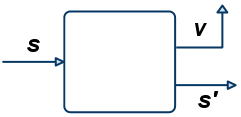
type State = ...The most basic form of function on this type is a state transformer (abbreviated by ST), which takes the current state as its argument, and produces a modified state as its result, in which the modified state reflects any side effects performed by the function:
type ST = State -> StateIn general, however, we may wish to return a result value in addition to updating the state. For example, a function for incrementing a counter may wish to return the current value of the counter. For this reason, we generalise our type of state transformers to also return a result value, with the type of such values being a parameter of the ST type:
data ST a = ST (State -> (a, State))
            deriving (Functor)

instance Monad ST where
  -- return :: a -> ST a
  return x  = ST (\st -> (x, st))

  -- >>=    :: ST a -> (a -> ST b) -> ST b
  ma >>= f  = ST (\st ->
                   let  (soma, ST st') = (ma st)
                        (somb, st'')   = (f soma st')
                   in
                      (somb, st''))

  -- >>=    :: ST a -> (a -> ST b) -> ST b
  tx1 >>= f = ST (\st -> let (v, st') = tx1 st in
                             tx2      = f v
                         in tx2 st')
Such functions can be depicted as follows, where s is the input state, s' is the output state, and v is the result value:
The state transformer may also wish to take argument values. However, there is no need to further generalise the ST type to take account of this, because this behaviour can already be achieved by exploiting currying. For example, a state transformer that takes a character and returns an integer would have type Char -> ST Int, which abbreviates the curried function type
Char -> State -> (Int, State)depicted by:
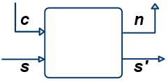
Returning to the subject of monads, it is now straightforward to make ST into an instance of a monadic type:
instance Monad ST where
   -- return :: a -> ST a
   return x  =  \s -> (x,s)

   -- (>>=)  :: ST a -> (a -> ST b) -> ST b
   st >>= f  =  \s -> let (x,s') = st s in f x s'
That is, return converts a value into a state transformer that simply returns that value without modifying the state:
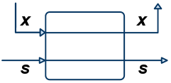
In turn, >>= provides a means of sequencing state transformers: st >>= f applies the state transformer st to an initial state s, then applies the function f to the resulting value x to give a second state transformer (f x), which is then applied to the modified state s' to give the final result:
Note that return could also be defined by return x s = (x,s). However, we prefer the above definition in which the second argument s is shunted to the body of the definition using a lambda abstraction, because it makes explicit that return is a function that takes a single argument and returns a state transformer, as expressed by the type a -> ST a: A similar comment applies to the above definition for >>=.
We conclude this section with a technical aside. In Haskell, types defined using the type mechanism cannot be made into instances of classes. Hence, in order to make ST into an instance of the class of monadic types, in reality it needs to be redefined using the data mechanism, which requires introducing a dummy constructor (called S for brevity):
> data ST0 a = S0 (State -> (a, State))
>              deriving (Functor)
It is convenient to define our own application function for this type, which simply removes the dummy constructor:
> apply0          :: ST0 a -> State -> (a, State)
> apply0 (S0 f) s0 = f s0
In turn, ST is now defined as a monadic type as follows:
>
> instance Monad ST0 where
>   -- return :: a -> ST0 a
>   return x   = S0 (\s -> (x, s))
>
>   -- (>>=)  :: ST0 a -> (a -> ST0 b) -> ST0 b
>   -- st >>= f   = S0 ( \s -> let (x, s') = apply0 st s in
>                           -- apply0 (f x) s'
>                   -- )
>
>   (S0 actA) >>= f = S0 ( \s -> let (xa, s')  = actA s
>                                    S0 actB   = f xa
>                                    (xb, s'') = actB s'
>                                in
>                                   (xb, s'')
> )(Aside: the runtime overhead of manipulating the dummy constructor S can be eliminated by defining ST using the newtype mechanism of Haskell, rather than the data mechanism.)
Intuitively, a value of type ST a (or ST0 a) is simply an action that returns an a value. The sequencing combinators allow us to combine simple actions to get bigger actions, and the apply0 allows us to execute an action from some initial state.
To get warmed up with the state-transformer monad, lets write a simple sequencing combinator
(>>) :: Monad m => m a -> m b -> m bwhich, in a nutshell, a1 >> a2 takes the actions a1 and a2 and returns the mega action which is a1-then-a2-returning-the-value-returned-by-a2.
Which is a valid implementation of >> ?
do x1 <- e1 x2 <- e2 e
e1 >>= 1 -> e2 >>= 2 -> e
do e1 e2 e
e1 >> e2 >> e e1 >>= _ -> e2 >>= _ -> e
-- a
a1 >> a2 = a1 >>= (\x -> a2 x)

-- b
a1 >> a2 = (a1, a2)

-- c
a1 >> a2 = a1 >>= (\_ -> a2)

-- d
a1 >> a2 = a1 >>= (\_ -> return a2)

-- e
a1 >> a2 = (a1, return a2)Next, lets see how to implement a “global counter” in Haskell, by using a state transformer, in which the internal state is simply the next integer
> type State = IntIn order to generate the next integer, we define a special state transformer that simply returns the current state as its result, and the next integer as the new state:
> fresh :: ST0 Int
> fresh =  S0 (\n -> (n, n+1))
>
> freshName :: ST0 String
> freshName =  S0 (\n -> ("burrito" ++ show n, n + 1))
Note that fresh is a state transformer (where the state is itself just Int), that is an action that happens to return integer values.
Recall that:
fresh           :: ST0 Int
fresh           =  S0 (\n -> (n, n+1))

apply0          :: ST0 a -> State -> (a, State)
apply0 (S0 f) x = f x
Consider the function wtf1 defined as:
> wtf1 = fresh >>= \_ ->
>          fresh >>= \_ ->
>            fresh >>= \_ ->
>              freshName
What does this return?
ghci> apply0 wtf1 0(3, 4)(0, 4)(3, 3)(4, 4)4
Indeed, we are just chaining together four fresh actions to get a single action that “bumps up” the counter by 4. That is, the following are equivalent:
wtf1 = fresh >>= \_ ->
         fresh >>= \_ ->
           fresh >>= \_ ->
             fresh

wtf1 = do fresh
          fresh
          fresh
          fresh

wtf1 = fresh >> fresh >> fresh >> fresh
Now, the >>= sequencer is kind of like >> only it allows you to “remember” intermediate values that may have been returned. Similarly,
return :: a -> ST0 atakes a value x and yields an action that doesnt actually transform the state, but just returns the same value x. So, putting things together, how do you think this behaves?
Recall:
fresh           :: ST0 Int
fresh           =  S0 (\n -> (n, n+1))

apply0          :: ST0 a -> State -> (a, State)
apply0 (S0 f) x = f x

return          :: a -> ST0 a
return x        = S0 (\n -> (x, n))
> wtf2 = fresh >>= \n1 ->
> freshName >>= \n2 ->
> fresh >>
> fresh >>
> return (n1, n2)What does the following evaluate to?
ghci> apply0 wtf2 04([3, 4], 4)((0, "nurrito1"), 4)[0, 1][3, 4]
Of course, the do business is just nice syntax for the above:
> wtf3 = do n1 <- fresh
>           n2 <- fresh
>           fresh
>           fresh
>           return [n1, n2]
is just like wtf2.
By way of an example of using the state monad, let us define a type of binary trees whose leaves contains values of some type a:
> data Tree a = Leaf a
>             | Node (Tree a) (Tree a)
>             deriving (Eq, Show)
Here is a simple example:
> tree :: Tree Char
> tree =  Node (Node (Leaf 'a') (Leaf 'b')) (Leaf 'c')
Now consider the problem of defining a function that labels each leaf in such a tree with a unique or “fresh” integer, for example, returning the following:
> tree' = Node (Node (Leaf ('a', 0)) (Leaf ('b', 1))) (Leaf ('c', 2))This can be achieved by taking the next fresh integer as an additional argument to the function, and returning the next fresh integer as an additional result, for instance, as shown below:
Note that the programmer does not have to worry about the tedious and error-prone task of dealing with the plumbing of fresh labels, as this is handled automatically by the state monad.
Finally, we can now define a function that labels a tree by simply applying the resulting state transformer with zero as the initial state, and then discarding the final state:
> label  :: Tree a -> Tree (a, Int)
> label t = fst (apply0 (mlabel t) 0)
For example, label tree gives the following result:
ghci> label tree
Node (Node (Leaf ('a', 0)) (Leaf ('b',1))) (Leaf ('c', 2))Define a function app :: (State -> State) -> ST0 State, such that fresh can be redefined by fresh = app (+1).
Define a function run :: ST0 a -> State -> a, such that label can be redefined by label t = run (mlabel t) 0.
Often, the state that we want to have will have multiple components, eg multiple variables whose values we might want to update. This is easily accomplished by using a different type for State above, for example, if we want two integers, we might use the definition
type State = (Int, Int)and so on.
Since state is a handy thing to have, the standard library includes a module Control.Monad.State that defines a parameterized version of the state-transformer monad above. (You will use this library in your next HW.)
We will only allow clients to use the functions declared below
module MyState (ST, get, put, apply) whereThe type definition for a generic state transformer is very simple:
> data ST s a = S (s -> (a, s)) deriving (Functor)is a parameterized state-transformer monad where the state is denoted by type s and the return value of the transformer is the type a. We make the above a monad by declaring it to be an instance of the monad typeclass
> instance Monad (ST s) where
>   return x   = S (\s -> (x, s))
>   st >>= f   = S (\s -> let (x, s') = apply st s
>                         in apply (f x) s')
where the function apply is just
> apply :: ST s a -> s -> (a, s)
> apply (S f) x = f xSince our notion of state is generic, it is useful to write a get and put function with which one can access and modify the state. We can easily get the current state via
> -- data ST s a = S (s -> (a, s)) deriving (Functor)
> get :: ST s s
> get = S (\s -> (s, s))
>
> put :: s -> ST s ()
> put s' = S (\_ -> ((), s'))
>
> -- fresh0 :: ST0 Int
> -- fresh0 = S0 (\n -> (n, n + 1))
>
>
> data Mem = Mem { sCount :: Int, sMap :: Map Char Int }
>
> newChar :: Char -> ST Mem Int
> newChar c = do
>   m    <- get
>   let i = 1 + sCount m
>   put (m { sCount = i
>          , sMap   = M.insert c i (sMap m) })
>   return i
>
> freshF :: Char -> ST Mem Int
> freshF c = do
>   m <- get
>   case M.lookup c (sMap m)  of
>     Just n  -> return n
>     Nothing -> newChar c
>
> foo :: Int -> ST Int String
>
> bar :: Int -> ST Mem String
>
>
> labelF :: Tree Char -> ST Mem (Tree (Char, Int))
> labelF (Leaf x)   =  do n <- freshF x
>                         return (Leaf (x, n))
> labelF (Node l r) =  do l'  <- labelF l
>                         r' <- labelF r
>                         return (Node l' r')
What is the TYPE of get ?
That is, get denotes an action that leaves the state unchanged, but returns the state itself as a value. What do you think the type of get is?
Dually, to modify the state to some new value s' we can write the function
> put s' = S (\_ -> ((), s'))We can use it like this…
> realfresh :: ST Int Int
> realfresh = do n <- get
>                put (n+1)
>                return n
>
> tuesday :: ST Int (Int, Int, Int)
> tuesday = do n1 <- realfresh
>              n2 <- realfresh
>              n3 <- realfresh
>              return (n1, n2, n3)
which denotes an action that ignores (ie blows away the old state) and replaces it with s'. Note that the put s' is an action that itselds yields nothing (that is, merely the unit value.)
Let us use our generic state monad to rewrite the tree labeling function from above. Note that the actual type definition of the generic transformer is hidden from us, so we must use only the publicly exported functions: get, put and apply (in addition to the monadic functions we get for free.)
Recall the action that returns the next fresh integer. Using the generic state-transformer, we write it as:
> freshS :: ST Int Int
> freshS = do n <- get
>             put (n+1)
>             return n
Now, the labeling function is straightforward
> mlabelS :: Tree a -> ST Int (Tree (a,Int))
> mlabelS (Leaf x)   =  do n <- freshS
>                          return (Leaf (x, n))
> mlabelS (Node l r) =  do l' <- mlabelS l
>                          r' <- mlabelS r
>                          return (Node l' r')
Easy enough!
ghci> apply (mlabelS tree) 0
(Node (Node (Leaf ('a', 0)) (Leaf ('b', 1))) (Leaf ('c', 2)), 3)
We can execute the action from any initial state of our choice
ghci> apply (mlabelS tree) 1000
(Node (Node (Leaf ('a',1000)) (Leaf ('b',1001))) (Leaf ('c',1002)),1003)
Now, whats the point of a generic state transformer if we can’t have richer states. Next, let us extend our fresh and label functions so that
Thus, our state will now have two elements, an integer denoting the next fresh integer, and a Map a Int denoting the number of times each leaf value appears in the tree.
> data MySt a = M { index :: Int
>                 , freq  :: Map a Int }
>               deriving (Eq, Show)
We write an action that returns the next fresh integer as
> freshM = do
>   s     <- get
>   let n  = index s
>   put $ s { index = n + 1 }
>   return n
Similarly, we want an action that updates the frequency of a given element k
> updFreqM k = do
>   s    <- get
>   let f = freq s
>   let n = findWithDefault 0 k f
>   put $ s {freq = insert k (n + 1) f}
And with these two, we are done
> mlabelM (Leaf x)   =  do updFreqM x
>                          n <- freshM
>                          return $ Leaf (x, n)
>
> mlabelM (Node l r) =  do l' <- mlabelM l
>                          r' <- mlabelM r
>                          return $ Node l' r'
Now, our initial state will be something like
> initM = M 0 emptyand so we can label the tree
> tree2 =  Node (Node (Leaf 'a') (Leaf 'b'))
> (Node (Leaf 'a') (Leaf 'c'))ghci> let tree2 = Node tree tree
ghci> let (tree2', s) = apply (mlabelM tree) $ M 0 empty
ghci> tree2'
Node (Node (Leaf ('a', 0)) (Leaf ('b', 1)))
(Node (Leaf ('a', 2)) (Leaf ('c', 3)))
ghci> s
M {index = 4, freq = fromList [('a',2),('b',1),('c',1)]}In short, ST makes global variables really easy.
Recall that interactive programs in Haskell are written using the type IO a of “actions” that return a result of type a, but may also perform some input/output. A number of primitives are provided for building values of this type, including:
return  :: a -> IO a
(>>=)   :: IO a -> (a -> IO b) -> IO b
getChar :: IO Char
putChar :: Char -> IO ()
The use of return and >>= means that IO is monadic, and hence that the do notation can be used to write interactive programs. For example, the action that reads a string of characters from the keyboard can be defined as follows:
getLine :: IO String
getLine =  do x <- getChar
              if x == '\n' then
                 return []
              else
                 do xs <- getLine
                    return (x:xs)
It is interesting to note that the IO monad can be viewed as a special case of the state monad, in which the internal state is a suitable representation of the “state of the world”:
   type World = ...

   type IO a  = World -> (a, World)
That is, an action can be viewed as a function that takes the current state of the world as its argument, and produces a value and a modified world as its result, in which the modified world reflects any input/output performed by the action. In reality, Haskell systems such as Hugs and GHC implement actions in a more efficient manner, but for the purposes of understanding the behaviour of actions, the above interpretation can be useful.
An important benefit of abstracting out the notion of a monad into a single typeclass, is that it then becomes possible to define a number of useful functions that work in an arbitrary monad.
We’ve already seen this in the pairs function
> pairs xs ys = do
>   x <- xs
>   y <- ys
>   return (x, y)
What do you think the type of the above is ? (I left out an annotation deliberately!)
ghci> :type pairs
pairs: (monad m) => m a -> m b -> m (a, b)
It takes two monadic values and returns a single paired monadic value. Be careful though! The function above will behave differently depending on what specific monad instance it is used with! If you use the Maybe monad
ghci> pairs (Nothing) (Just 'a')
Nothing

ghci> pairs (Just 42) (Nothing)
Just 42

ghci> pairs (Just 2) (Just 'a')
Just (2, a)
this generalizes to the list monad
ghci> pairs [] ['a']
[]

ghci> pairs [42] []
[]

ghci> pairs [2] ['a']
[(2, a)]

ghci> pairs [1,2] "ab"
[(1,'a') , (2, 'a'), (1, 'b'), (2, 'b')]
However, the behavior is quite different with the IO monad
ghci> pairs getChar getChar
40('4','0')What is the type of foo defined as:
> foo f z = do x <- z
>              return (f x)
(a -> b) -> Maybe a -> Maybe b(a -> b) -> IO a -> IO b(a -> b) -> [a] -> [b](Monad m) => (a -> b) -> m a -> m b
Whoa! This is actually very useful, because in one-shot we’ve defined a map function for every monad type!
ghci> foo (+1) [0,1,2]
[1, 2, 3]

ghci> foo (+1) (Just 10)
Just 11

ghci> foo (+1) Nothing
Nothing
Indeed, we can make this explicit by telling Haskell that every Monad also is a Functor:
instance (Monad m) => (Functor m) where
  fmap :: (a -> b) -> m a -> m b
  fmap f z = do x <- z
return (f x)Consider the function baz defined as:
> baz mmx = do mx <- mmx
>              x  <- mx
>              return x
What does baz [[1, 2], [3, 4]] return ?
[1, 3], [1, 4], [2, 3], [2, 4]][1, 2, 3, 4][[1, 3], [2, 4]][]This above notion of concatenation generalizes to any monad:
> join    :: Monad m => m (m a) -> m a
> join mmx = do mx <- mmx
>               x  <- mx
>               return x
As a final example, we can define a function that transforms a list of monadic expressions into a single such expression that returns a list of results, by performing each of the argument expressions in sequence and collecting their results:
sequence          :: Monad m => [m a] -> m [a]
sequence []       =  return []
sequence (mx:mxs) =  do x  <- mx
                        xs <- sequence mxs
return (x:xs)It is sometimes useful to sequence two monadic expressions, but discard the result value produced by the first:
(>>)     :: Monad m => m a -> m b -> m b
mx >> my =  do _ <- mx
               y <- my
               return y
For example, in the state monad the >> operator is just normal sequential composition, written as ; in most languages.
Indeed, in Haskell the entire do notation with or without ; is just syntactic sugar for >>= and >>. For this reason, we can legitimately say that Haskell has a programmable semicolon.
Define liftM and join more compactly by using >>=.
Explain the behaviour of sequence for the maybe monad.
Define another monadic generalisation of map:
mapM :: Monad m => (a -> m b) -> [a] -> m [b]foldM :: Monad m => (a -> b -> m a) -> a -> [b] -> m aEarlier we mentioned that the notion of a monad requires that the return and >>= functions satisfy some simple properties. The first two properties concern the link between return and >>=:
return x >>= f  =  f x	--	(1)

mx >>= return   =  mx	--	(2)
Intuitively, equation (1) states that if we return a value x and then feed this value into a function f, this should give the same result as simply applying f to x. Dually, equation (2) states that if we feed the results of a computation mx into the function return, this should give the same result as simply performing mx. Together, these equations express — modulo the fact that the second argument to >>= involves a binding operation — that return is the left and right identity for >>=.
The third property concerns the link between >>= and itself, and expresses (again modulo binding) that >>= is associative:
(mx >>= f) >>= g = mx >>= (\x -> (f x >>= g)) -- (3)Note that we cannot simply write mx >>= (f >>= g) on the right hand side of this equation, as this would not be type correct.
As an example of the utility of the monad laws, let us see how they can be used to prove a useful property of the liftM function from the previous section, namely that it distributes over the composition operator for functions, in the sense that:
liftM (f . g) = liftM f . liftM gThis equation generalises the familiar distribution property of map from lists to an arbitrary monad. In order to verify this equation, we first rewrite the definition of liftM using >>=: That is, we change the definition:
liftM f mx = do { x <- mx ; return (f x) }into
liftM f mx = mx >>= \x -> return (f x)Now the distribution property can be verified as follows:
(liftM f . liftM g) mx
   = {-   applying . -}
     liftM f (liftM g mx)
   = {-   applying the second liftM -}
     liftM f (mx >>= \x -> return (g x))
   = {-   applying liftM -}
     (mx >>= \x -> return (g x)) >>= \y -> return (f y)
   = {-   equation (3) -}
     mx >>= (\z -> (return (g z) >>= \y -> return (f y)))
   = {-   equation (1) -}
     mx >>= (\z -> return (f (g z)))
   = {-   unapplying . -}
     mx >>= (\z -> return ((f . g) z)))
   = {-   unapplying liftM -}
liftM (f . g) mxShow that the maybe monad satisfies equations (1), (2) and (3).
Given the type
> data Expr a = Var a | Val Int | Add (Expr a) (Expr a)of expressions built from variables of type a, show that this type is monadic by completing the following declaration:
   instance Monad Expr where
      -- return       :: a -> Expr a
      return x         = ...

      -- (>>=)        :: Expr a -> (a -> Expr b) -> Expr b
      (Var a)   >>= f  = ...
      (Val n)   >>= f  = ...
      (Add x y) >>= f  = ...
Hint: think carefully about the types involved. With the aid of an example, explain what the >>= operator for this type does.
The subject of monads is a large one, and we have only scratched the surface here. If you are interested in finding out more, two suggestions for further reading would be to look at “monads with a zero a plus” (which extend the basic notion with two extra primitives that are supported by some monads), and “monad transformers” (which provide a means to combine monads.) For example, see sections 3 and 7 of the following article, which concerns the monadic nature of functional parsers For a more in-depth exploration of the IO monad, see Simon Peyton Jones’ excellent article on the “awkward squad”